Intro to Rcpp

class: middle, right, title-slide

# Intro to Rcpp
## Oslo UseR! Group
### Øystein Sørensen
### 2019/02/06

---

layout: true
    
<div class="my-sidebar"></div>

---

# Short Bio

- Associate professor at the University of Oslo.

- R user since 2011.

- Author of two packages which use Rcpp.

---
# Outline

--
1. Understanding the speed of R.

- Stuff you can do before trying Rcpp.
  
--

2. When is R slow compared to C/C++?

3. Introduction to Rcpp

- Data types, how to write functions.
  
  - Some examples.
--

4. Extensions

- RcppArmadillo, RcppParallel, RcppGSL, ...

---
# Packages

```r
library(microbenchmark)

library(tidyverse)

library(Rcpp)
```

---
class: inverse, middle, center

# Understanding the speed of R

---

# Compiled vs Interpreted Languages
.pull-left[
- R is an interpreted language, i.e., you can write commands in a console:

```r
a <- 1
v <- rnorm(10)
```

- C, C++, and Fortran are compiled languages. You must do (in the shell):

```bash
g++ script.cpp
```
]
--
.pull-right[
- From [the internet](http://www.vanguardsw.com/dphelp4/dph00296.htm):

> With a compiled language, code you enter is reduced to a set of machine-specific instructions [...]. Compiled programs generally run faster than interpreted ones because interpreted programs must be reduced to machine instructions at runtime.
]

---
# What about R?

- The functions in base R are written in C, Fortran, and R itself.

- C functions can be recognized with a call to `.Primitive` or `.Internal`.

```r
sum
```

```
## function (..., na.rm = FALSE)  .Primitive("sum")
```

- If you are really interested:

```r
library(pryr)

show_c_source(.Primitive(sum(x)))
```

---

```r
mean.default
```

```
## function (x, trim = 0, na.rm = FALSE, ...) 
## {
##     if (!is.numeric(x) && !is.complex(x) && !is.logical(x)) {
##         warning("argument is not numeric or logical: returning NA")
##         return(NA_real_)
##     }
##     if (na.rm) 
##         x <- x[!is.na(x)]
##     if (!is.numeric(trim) || length(trim) != 1L) 
##         stop("'trim' must be numeric of length one")
##     n <- length(x)
##     if (trim > 0 && n) {
##         if (is.complex(x)) 
##             stop("trimmed means are not defined for complex data")
##         if (anyNA(x)) 
##             return(NA_real_)
##         if (trim >= 0.5) 
##             return(stats::median(x, na.rm = FALSE))
##         lo <- floor(n * trim) + 1
##         hi <- n + 1 - lo
##         x <- sort.int(x, partial = unique(c(lo, hi)))[lo:hi]
##     }
##     .Internal(mean(x))
## }
## <bytecode: 0x7fac42f0eae8>
## <environment: namespace:base>
```

---
# Vectorization

- ... is the key to utilizing functions written in C, and hence writing fast R code.

- Consider finding the maximum of each row of this matrix:

```r
head(mat)
```

```
##             [,1]       [,2]       [,3]
## [1,]  1.08722580 -0.3796144  0.4512066
## [2,]  1.44834102  1.2511557  0.3020791
## [3,] -1.77562674  1.8573989  0.9553197
## [4,]  0.14165171  1.4253457  0.1129406
## [5,]  0.03148697  0.1671864  0.1811391
## [6,]  1.14378308  0.8541135 -1.7144960
```

```r
dim(mat)
```

```
## [1] 100000      3
```

---
# Finding Row-Wise Maximum

```r
loop_fun <- function(mat) {
  result <- numeric(nrow(mat))
  for(i in seq(1, nrow(mat), by = 1)) result[[i]] <- max(mat[i, ])
  result
}
```

```r
apply_fun <- function(mat) apply(mat, 1, max)
```

```r
pmax_fun <- function(mat) pmax(mat[, 1], mat[, 2], mat[, 3])
```

```r
library(matrixStats)
matStats_fun <- function(mat) rowMaxs(mat)
```

```r
identical(loop_fun(mat), apply_fun(mat)) && 
  identical(apply_fun(mat), pmax_fun(mat)) && 
  identical(pmax_fun(mat), matStats_fun(mat))
```

```
## [1] TRUE
```

---
# Which is faster?

```r
microbenchmark(
  loop_fun(mat), apply_fun(mat), pmax_fun(mat), matStats_fun(mat)
) %>% 
  print(signif = 3)
```

```
## Unit: milliseconds
##               expr   min    lq   mean median     uq    max neval
##      loop_fun(mat) 58.60 66.80  80.10  76.50  87.40 178.00   100
##     apply_fun(mat) 80.20 93.70 114.00 111.00 126.00 213.00   100
##      pmax_fun(mat)  1.76  1.99   2.61   2.54   3.11   9.22   100
##  matStats_fun(mat)  1.18  1.32   1.55   1.51   1.73   2.89   100
```

- `apply` and `for` loop work one row at a time.

- `pmax` sends all vectors directly to C, through `.Internal`.

- `matrixStats::rowMaxs` uses C code, tailored to the problem.

---

# Sometimes you cannot vectorize
.pull-left[

- Model hippocampus volume as a function of age:

```r
library(mgcv); library(voxel)
fit <- gam(Value ~ s(Age), data = df)
```

- Volume is maximal at 22 years age.

- What is the confidence interval of the age at maximum?

]
.pull-right[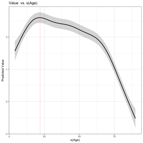
![](presentation_files/figure-html/unnamed-chunk-18-1.png)
]

---

# Sometimes you cannot vectorize
.pull-left[
- Sample 10000 curves from posterior distribution. Find the age at maximum for each.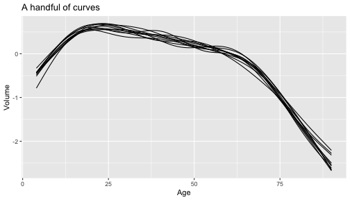

![](presentation_files/figure-html/unnamed-chunk-20-1.png)
]
--
.pull-right[
- We have a 10000 X 87 matrix.

```r
fits[1:4, 22:25]
```

```
##          Age25     Age26     Age27     Age28
## Sim1 0.5421727 0.5310547 0.5186932 0.5053755
## Sim2 0.6158313 0.6004825 0.5816612 0.5607164
## Sim3 0.6475296 0.6319094 0.6141901 0.5949870
## Sim4 0.6585477 0.6591823 0.6569978 0.6524447
```

- Find the **index** of the maximum in each row, the R way:

```r
maxima <- apply(fits, 1, which.max)
```

]

---

# Sometimes you cannot vectorize
.pull-left[
- We get a nice posterior distribution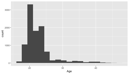

![](presentation_files/figure-html/unnamed-chunk-23-1.png)
]
--
.pull-right[
- And the confidence interval

```r
quantile(df$Age[maxima], 
         probs = c(0.025, 0.975))
```

```
##  2.5% 97.5% 
##    18    36
```
]

---

# Alternative to apply
.pull-left[
- But we can be faster!

- Rcpp function looping through the matrix, row by row:

```cpp
#include <Rcpp.h>
using namespace Rcpp;

// [[Rcpp::export]]
IntegerVector cpp_which(NumericMatrix m){
  int n = m.nrow();
  IntegerVector v(n);
  for(int i = 0; i < n; ++i){
    v(i) = which_max(m(i, _)) + 1;
  }
  return v;
}
```
]
--
.pull-right[

```r
all.equal(
  as.integer(apply(fits, 1, which.max)),
  cpp_which(fits)
)
```

```
## [1] TRUE
```
]

---
# How fast?

```r
microbenchmark(
  apply(fits, 1, which.max),
  cpp_which(fits)
) %>% 
  print(signif = 3)
```

```
## Unit: milliseconds
##                       expr   min    lq  mean median    uq    max neval
##  apply(fits, 1, which.max) 31.50 40.90 51.50  48.10 58.20 171.00   100
##            cpp_which(fits)  2.62  3.28  3.47   3.42  3.66   4.23   100
```

---
class: inverse, middle, center

# When is R slow compared to C/C++?

---
# When is R slow compared to C/C++?

- When you have to repeatedly call a function in a loop.

- Remember that `apply` is a loop
  
  - And so are the `map` family of functions from `purrr`.
  
- Ways to fix it:

1. Search CRAN for a package that already does the job.
  
  2. Code it yourself.
  
- But also, *slow compared to C++* can often be more than fast enough.

---
class: inverse, middle, center

# Introduction to Rcpp

---
# Introduction to Rcpp

- Rcpp has data types that:

- Facilitate data exchange between R and C++.
  
  - Make C++ programming feel almost like R.

- [Rcpp for Everyone](https://teuder.github.io/rcpp4everyone_en/) has the following overview (which I simplified):

---

# Rcpp Vector Example
.pull-left[
- Add two vectors elementwise:

```cpp
#include <Rcpp.h>
using namespace Rcpp;

// [[Rcpp::export]]
NumericVector add(NumericVector vec1, 
                  NumericVector vec2){
  return vec1 + vec2;
}
```
]
--
.pull-right[
- In a script, put code in `file.cpp` and run `sourceCpp("file.cpp")`.

- In RMarkdown, just specify that chunk is running `Rcpp`.
]

---
# Rcpp Vector Example

```r
add(1.0, 0.2)
```

```
## [1] 1.2
```

```r
add(1:10, rnorm(10))
```

```
##  [1]  0.7315609  1.4820625  3.1129064  2.6486520  4.3531346  7.8076578
##  [7]  6.1463096  9.2909798  9.7332486 10.5931057
```

---
# Rcpp Vector Example
- How does the code below compare to R?

```r
add(1:3, 1:4)
```

```
## [1] 2 4 6
```

```r
add(1:4, 1:3)
```

```
## [1] 2 4 6 4
```

---
# Rcpp Vector Example

- Safer version?

```cpp
#include <Rcpp.h>
using namespace Rcpp;

// [[Rcpp::export]]
NumericVector add(NumericVector vec1, NumericVector vec2){
  if(vec1.length() != vec2.length()) {
    warning("Vectors not of same length.\n");
  }
  
  return vec1 + vec2;
}
```

```r
add(1:3, 1:4)
```

```
## Warning in add(1:3, 1:4): Vectors not of same length.
```

```
## [1] 2 4 6
```

---

# Dataframes
.pull-left[
- Create a dataframe from two vectors.

```cpp
#include <Rcpp.h>
using namespace Rcpp;

// [[Rcpp::export]]
DataFrame rcpp_df(NumericVector v1, 
                  NumericVector v2){
    
    DataFrame df = DataFrame::create( 
      Named("V1") = v1, Named("V2") = v2);
    
    return df;
}
```
]
--
.pull-right[

```r
rcpp_df(1:2, 2:1)
```

```
##   V1 V2
## 1  1  2
## 2  2  1
```

```r
rcpp_df(1:2, 1:4)
```

```
##   V1 V2
## 1  1  1
## 2  2  2
## 3  1  3
## 4  2  4
```

```r
rcpp_df(1:2, 1:3)
```

```
## Error in rcpp_df(1:2, 1:3): Could not convert using R function: as.data.frame.
```
]

---

# Dataframes
.pull-left[
- Dataframes contain *references* two their constituent vectors.

```cpp
#include <Rcpp.h>
using namespace Rcpp;

// [[Rcpp::export]]
DataFrame rcpp_df(NumericVector v1, 
                  NumericVector v2){
    
  DataFrame df = DataFrame::create( 
    Named("V1") = v1, Named("V2") = v2);
  
  v1 = v1 + v2;
    
  return df;
}
```
]
--
.pull-right[

```r
rcpp_df(1:2, 1:2)
```

```
##   V1 V2
## 1  2  1
## 2  4  2
```

- Copy the whole vector with `clone()`

```cpp
DataFrame df = DataFrame::create( 
    Named("V1") = clone(v1), 
    Named("V2") = clone(v2));
```

]

---
class: inverse, middle, center

# A Real Example

---
# Disclaimer

- The intention of the following slides is to illustrate Rcpp. The algorithms used are complete overkill for this toy problem.

---

# Bayesian Linear Regression
.pull-left[
- Modified diamonds dataset from ggplot2:

```r
df
```

```
## # A tibble: 100 x 2
##     price volume
##     <dbl>  <dbl>
##  1 -0.637 -0.550
##  2  0.637  1.30 
##  3 -0.815 -0.944
##  4 -0.776 -0.986
##  5  2.17   1.46 
##  6 -0.451 -0.202
##  7 -0.280 -0.127
##  8 -0.789 -0.812
##  9  0.736  0.365
## 10 -0.655 -0.647
## # … with 90 more rows
```

]
--
.pull-right[
- We want to predict the price of a diamond given its volume.

`$$y = \beta v + \epsilon$$`
- A frequentist model for this would be

```r
lm(price ~ volume, data = df)
```

- This does not let us incorporate prior information, which we sometimes have.
]

---

# Bayesian Linear Regression
.pull-left[
- We have prior knowledge telling us that `$\beta$` is approximately normally distributed with mean 1 and standard deviation 1.

- Pretend we know `$\sigma = 0.5$`.

- Our full model is hence:

`$$y = \beta v + \epsilon$$` `$$f(\epsilon) = N(0, \sigma^{2})$$` `$$f(\beta) = N(1, 1)$$`
- Our target is `$$f(\beta | x, y)$$`

]
.pull-right[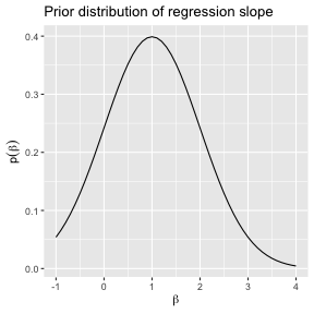
![](presentation_files/figure-html/unnamed-chunk-43-1.png)
]

---

# Metropolis Algorithm

- In general, computing the posterior distribution of `$\beta$` requires use of the Metropolis algorithm, **which is a loop we cannot avoid**.

- It goes like this (almost):

1. Initialize `$\beta^{1}$`.

2. For `$i=2,\dots,N$`:

i. Sample `$\beta'$` from proposal distribution.

ii. Compute the ratio `$r = \frac{p(\beta') l(\beta'|x,y)}{p(\beta) l(\beta|x,y)}$`, where `$l()$` is the log-likelihood of the model.
  
  iii. Sample a uniform number `$u \sim U(0, 1)$`.
  
  iv. If `$u < r$`, `$\beta^{i}=\beta^{i-1}$`, else `$\beta^{i}=\beta'$`.
  
3. In the end we have `$N$` samples from the posterior distribution `$p(\beta|x, y)$`.

---

# Metropolis Algorithm in R

```r
ratio_fun <- function(b_old, b_prop){
  exp(-(b_prop - 1)^2 - sum(((y - x * b_prop)^2 - (y - x * b_old)^2)/0.5^2) +
    (b_old - 1)^2)
}

r_metropolis <- function(x, y, nmc){
  beta <- c(0, numeric(nmc - 1))
  
  for(i in 2:nmc){
    beta_proposal <- rnorm(1, mean = beta[[i - 1]], sd = .05)
    ratio <- ratio_fun(b_old = beta[[i - 1]], b_prop = beta_proposal)
    beta[[i]] <- if_else(ratio > runif(1), beta_proposal, beta[[i - 1]])
  }
  return(beta)
}
```

---

# Metropolis Algorithm in R

```r
y <- as.numeric(df$price); 
x <- as.numeric(df$volume)
beta_posterior <- r_metropolis(x, y, 500)
```

![](presentation_files/figure-html/unnamed-chunk-46-1.png)

---
# Metropolis Algorithm

- Real applications have

- Missing data --> inner loops over all rows in each step
  
  - Mixtures (clustering) --> outer loops
  
  - Many parameters
  
- Hence need a large number of iterations

---
# Metropolis Algorithm in C++

```cpp
#include <Rcpp.h>
using namespace Rcpp;

double ratio_fun(double b_old, double b_prop, 
             NumericVector x, NumericVector y){
  return exp(-pow(b_prop - 1, 2) - sum(pow((y - x * b_prop), 2)/pow(0.5, 2)) + 
             pow(b_old - 1, 2) + sum(pow((y - x * b_old), 2)/pow(0.5, 2)));
}

// [[Rcpp::export]]
NumericVector cpp_metropolis(NumericVector x, NumericVector y, int nmc){
  NumericVector beta(nmc);
  
  for(int i = 1; i < beta.length(); ++i){
    double beta_proposal = R::rnorm(beta(i - 1), .05);
    double ratio = ratio_fun(beta(i - 1), beta_proposal, x, y);    
    if(ratio > R::runif(0, 1)){
      beta(i) = beta_proposal;
    } else {
      beta(i) = beta(i - 1);
    }
  }
  return beta;
}

```

---
# Metropolis Algorithm in C++

```r
beta_posterior = cpp_metropolis(x, y, 500) 
```

![](presentation_files/figure-html/unnamed-chunk-49-1.png)

---
# Comparative Timing

```r
microbenchmark(
  r_metropolis(x, y, 10000),
  cpp_metropolis(x, y, 10000)
)
```

```
## Unit: milliseconds
##                         expr        min         lq       mean    median
##    r_metropolis(x, y, 10000) 163.880972 172.832905 179.419026 176.65376
##  cpp_metropolis(x, y, 10000)   3.052297   3.209085   3.256571   3.22316
##          uq        max neval
##  180.714753 305.477435   100
##    3.288726   4.863254   100
```

---

# Posterior Distribution
.pull-left[

```r
df <- tibble(
  beta = cpp_metropolis(x, y, 10000)
  ) %>% 
  filter(row_number() > 1000)
```

![](presentation_files/figure-html/unnamed-chunk-52-1.png)
]
.pull-right[

- 95 % confidence interval:

```r
quantile(df$beta, probs = c(0.025, 0.975))
```

```
##      2.5%     97.5% 
## 0.8325933 0.9727383
```

- What is the probability that `$\beta$` is larger than 1.0?

```r
mean(df$beta > 1)
```

```
## [1] 0.001666667
```

]

---
class: inverse, middle, center

# Other Uses of Rcpp

---

# Using C++ Libraries

- Lucikly, a lot of algorithms are on CRAN.

- However, it does happen that what you need is only available in C/C++.

- Using Rcpp, you can create a wrapper to the C++ code, callable from R.

---

# Using C++ Libraries

- Trivial example, finding the length of a vector using `distance` from C++ standard template library.

```cpp
#include <Rcpp.h>
#include <iterator>
#include <vector>

using namespace Rcpp;
// [[Rcpp::plugins("cpp11")]]
// [[Rcpp::export]]
int cpp_length(IntegerVector v)
{
  return std::distance(v.begin(), v.end());
}
```

```r
cpp_length(1:4)
```

```
## [1] 4
```

---

# Using C++ Libraries

- If you want a package with impact, making an API to C++ code can be a good way to start.

- What is available in Python that you don't get in R?

---
# Useful Rcpp Tools

- RcppArmadillo

- Armadillo matrix library

- RcppParallel

- RcppGSL

- GNU Scientific Library
  
- Check out [http://www.rcpp.org/](http://www.rcpp.org/) for more.

---
# Summary and Advice

- Rcpp is an important part of you toolbox if you:

- Ever run into problems that cannot be vectorized.
  
  - And the pure R code is annoyingly slow.

- Learning C++ is hard

- Thus likely to be good for your brain, prevent dementia, etc.

--
- When writing code that should be shared with other, or parallelized, you must create a package.

- But this is the best practice for using R anyway!
  
---
class: inverse, middle, center

# Thank you, and good luck!